| Attribute | Type | Description |
|---|---|---|
| stime | Numeric | survival or follow-up time, in days |
| status | Numeric | dead or alive/censored; 0 (alive), 1 (dead) |
| treat | Nominal | treatment, either standard or test (chemotherapy); 1 (standard), 2 (test) |
| age | Numeric | patient age in years |
| Karn | Numeric | Karnofsky score of patient performance, on scale of 0 to 100 |
| diag | Numeric | patient time since diagnosis, measured at time of entry to trial, in months |
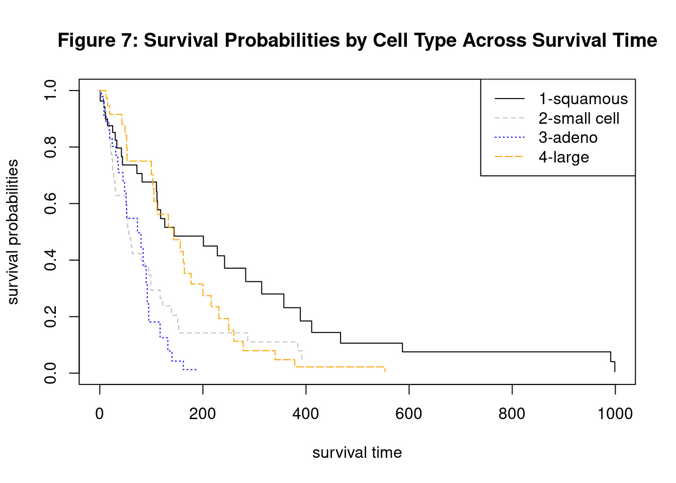
| cell | Nominal | one of four cell types; 1 (squamous), 2 (small cell), 3 (adeno), 4 (large) |
| prior | Nominal | denotes prior therapy; 10 (yes), 0 (no) |
Cox Proportional Hazards Model
Data Visualization
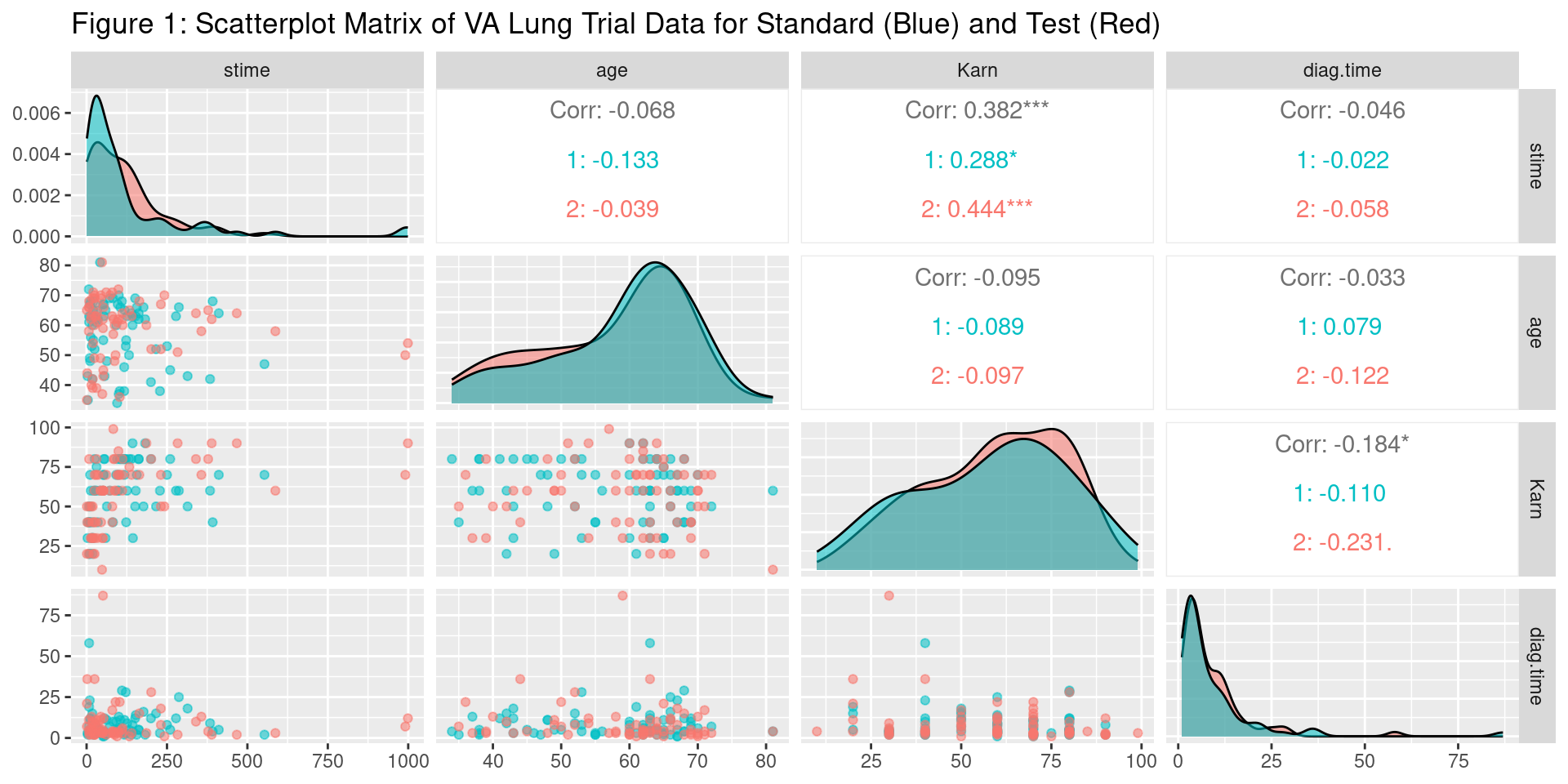
Distributions are roughly similar between standard and test treatment groups
Karnofsky and survival time seem positively correlated
#Create a scatter plot matrix using the GGally package
library(GGally)
library(tidyverse)
va_subset <- VA[, c("stime", "age", "Karn", "diag.time", "treat")]

ggpairs(va_subset, title = "Figure 1: Scatterplot Matrix of VA Lung Trial Data for Standard (Blue) and Test (Red)",
        columns = c("stime", "age", "Karn", "diag.time"), ggplot2::aes(color = treat),
        lower = list(continuous = "points", combo = "dot_no_facet", mapping = ggplot2::aes(color=treat, alpha = 0.8)),
        diag = list(continuous = wrap("densityDiag"), mapping = ggplot2::aes(color = treat, alpha = 0.1))) +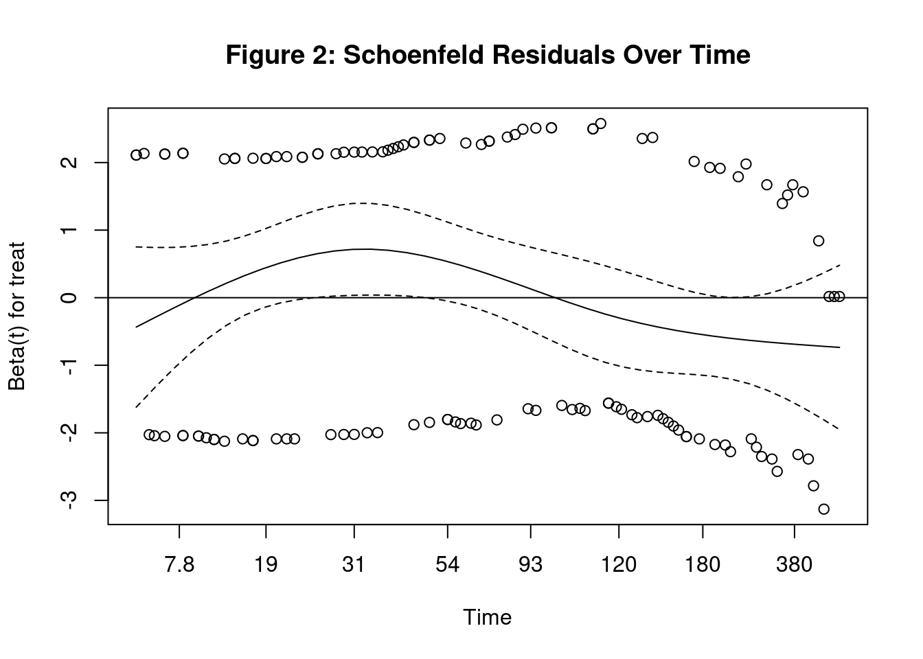
scale_color_manual(values = c("#00BFC4", "#F8766D"))1. Residuals vs Time Plot
PH assumption is valid when coefficient is constant over time.
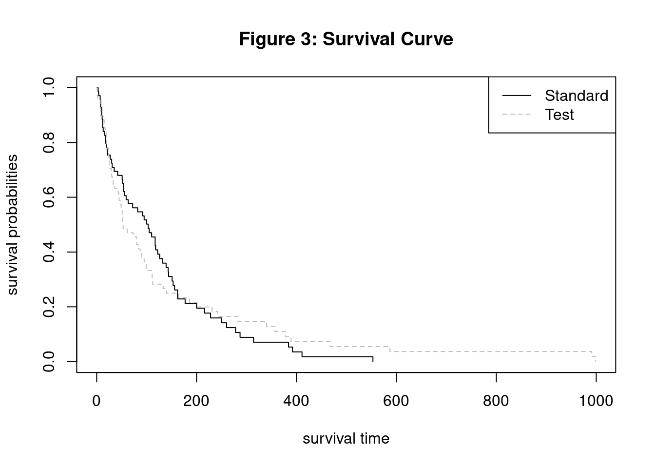
3. Survival Curves
Multiple Variable Cox Model
Call:
coxph(formula = Y ~ treat + age + Karn + diag.time + cell + prior,
    data = VA)

                coef  exp(coef)   se(coef)      z        p
treat2     2.946e-01  1.343e+00  2.075e-01  1.419  0.15577
age       -8.706e-03  9.913e-01  9.300e-03 -0.936  0.34920
Karn      -3.282e-02  9.677e-01  5.508e-03 -5.958 2.55e-09
diag.time  8.132e-05  1.000e+00  9.136e-03  0.009  0.99290
cell2      8.616e-01  2.367e+00  2.753e-01  3.130  0.00175
cell3      1.196e+00  3.307e+00  3.009e-01  3.975 7.05e-05
cell4      4.013e-01  1.494e+00  2.827e-01  1.420  0.15574
prior10    7.159e-02  1.074e+00  2.323e-01  0.308  0.75794

Likelihood ratio test=62.1  on 8 df, p=1.799e-10
n= 137, number of events= 128 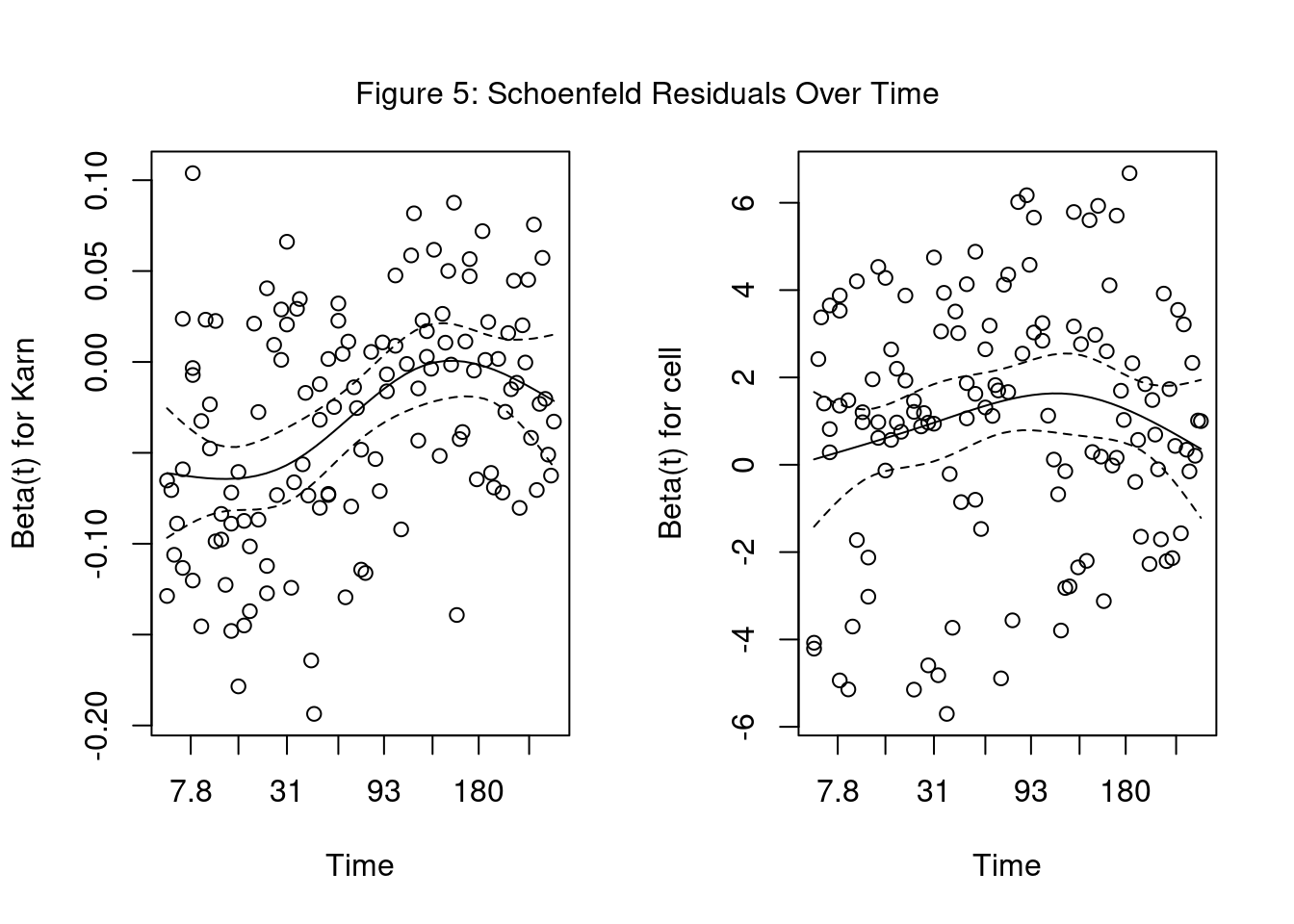
2. Stratified Cox model
Assumes a different baseline hazard function for each Cell Type.

where \[g = 1, 2, 3, 4 \text{ (number of cell types)}\]
Call:
coxph(formula = Y ~ treat + age + Karn + diag.time + strata(cell) +
    prior, data = VA)

               coef exp(coef)  se(coef)      z        p
treat2     0.285902  1.330962  0.210009  1.361    0.173
age       -0.011821  0.988249  0.009846 -1.201    0.230
Karn      -0.038262  0.962461  0.005932 -6.450 1.12e-10
diag.time -0.003439  0.996567  0.009075 -0.379    0.705
prior10    0.169069  1.184201  0.235667  0.717    0.473

Likelihood ratio test=44.27  on 5 df, p=2.042e-08
n= 137, number of events= 128 Final SE Cox model
Simplified the model to treat + Karn + cell.

where \[g = 1, 2, 3, 4 \text{ (number of cell types)}\] \[tgroup1 = 1 \text{ if } 0 \le t < 90 \] \[tgroup2 = 1 \text{ if } 90 \le t < 180 \] \[tgroup3 = 1 \text{ if } t \ge 180\]